Advanced Data Manipulation

Materials adapted from Adrien Osakwe, Larisa M. Soto and Xiaoqi Xie.

0. The “Base R” Struggle (A Scenario)

Imagine you have data from an experiment with a Control group and an Experimental group. Each group has 3 males and 3 females. You need to calculate the mean for each unique combination (Sex + Treatment).

The “Old” Way (Base R): You have to manually subset the data for every single combination, creating new variables each time.

# prepare demo dataset
set.seed(228)
demo_data <- data.frame(
  "Treatment" = c(rep("ctrl", 6), rep("experiment", 6)),
  "Sex" = c(rep("Male", 3), rep("Female", 3), rep("Male", 3), rep("Female", 3)),
  "Measurement" = c(sample(100:300, 12))
)

# Calculating means manually
Ctrl_M <- demo_data[which(demo_data$Treatment == "ctrl" & demo_data$Sex == "Male"), "Measurement"]
mean(Ctrl_M)
## [1] 213.3333

Ctrl_F <- demo_data[which(demo_data$Treatment == "ctrl" & demo_data$Sex == "Female"), "Measurement"]
mean(Ctrl_F)
## [1] 149.3333

Now imagine doing this for 10 treatments and 3 timepoints… you would have 60 variables!

There are packages that provide functions to streamline common operations on tabular data and make the code look nicer and cleaner. These packages are part of a broader family called tidyverse, for more information you can visit https://www.tidyverse.org/.

We will cover 5 of the most commonly used functions and combine them using pipes (%>%):

1. select() - used to extract data

2. filter() - to filter entries using logical vectors

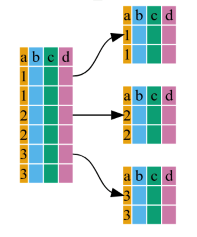
3. group_by() - to solve the split-apply-combine problem

4. summarize() - to obtain summary statistics

5. mutate() - to create new columns

1. The `tidyverse` Philosophy

To solve this “variable explosion,” we use dplyr. It is part of the tidyverse, a collection of R packages that are designed for data science and share a common grammar. The goal is to provide a consistent way to handle data frames. Instead of creating 60 intermediate objects, we create one Pipeline.

if (!require("gapminder", quietly = TRUE))
    install.packages("gapminder")
library(gapminder)

if (!require("dplyr", quietly = TRUE))
    install.packages("dplyr")
library(dplyr)

The Power of the Pipe (`%>%`)

The pipe operator is the secret sauce of dplyr. It takes the output of one function and “pipes” it directly into the next.

Think of it as the word “THEN”.

Why use the pipe?

Readability: Standard R code is nested like an onion: f(g(h(x))). You have to read from the inside out. With the pipe, you read from left to right (or top to bottom).
No “Intermediate Clutter”: You don’t have to save temp_data_1, temp_data_2, etc.
Easy Debugging: You can comment out one line of the pipe to see where the data “breaks.”

Comparisons: The Pipe vs. The Nest

The Nest (Hard to read):

# Hard to tell which argument belongs to which function
set.seed(228)
demo_data <- data.frame(
  "Treatment" = c(rep("ctrl", 6), rep("experiment", 6)),
  "Sex" = c(rep("Male", 3), rep("Female", 3), rep("Male", 3), rep("Female", 3)),
  "Measurement" = c(sample(100:300, 12))
)

as.data.frame(summarise(dplyr::group_by(demo_data, Treatment, Sex), Mean = mean(Measurement)))

   Treatment    Sex     Mean
1       ctrl Female 149.3333
2       ctrl   Male 213.3333
3 experiment Female 167.0000
4 experiment   Male 136.0000

The Pipe (Easy to read):

# Step-by-step logic
demo_data %>% 
  dplyr::group_by(Treatment, Sex) %>% 
  summarise(
    Mean = mean(Measurement),
    SD   = sd(Measurement),
    .groups  = "drop"
  ) %>% 
  as.data.frame()

   Treatment    Sex     Mean       SD
1       ctrl Female 149.3333 11.06044
2       ctrl   Male 213.3333 60.45108
3 experiment Female 167.0000 19.46792
4 experiment   Male 136.0000 24.75884

Note

Keyboard Shortcut:
- Windows/Linux: Ctrl + Shift + M
- Mac: Cmd + Shift + M
Fact: The pipe introduced in the magrittr package (2014) and popularized by dplyr (magrittr package was named after the artist René Magritte, famous for the “This is not a pipe” painting).
Modern R: Since R 4.1.0, there is a built-in pipe |>. It works similarly but has a few more restrictions (like requiring parentheses after every function).

2. The Core `dplyr` Verbs

2.1 `select()`: Picking Columns

Use select() when you only want specific variables (columns) from your dataset. Think of it as a logical sieve: you define the criteria, and only the rows that meet those conditions pass through.

# Select specific columns
gapminder %>% 
  dplyr::select(year, country, gdpPercap) %>% 
  head()
## # A tibble: 6 × 3
##    year country     gdpPercap
##   <int> <fct>           <dbl>
## 1  1952 Afghanistan      779.
## 2  1957 Afghanistan      821.
## 3  1962 Afghanistan      853.
## 4  1967 Afghanistan      836.
## 5  1972 Afghanistan      740.
## 6  1977 Afghanistan      786.

# Remove a column using the minus sign
gapminder %>% 
  dplyr::select(-continent) %>% 
  head()
## # A tibble: 6 × 5
##   country      year lifeExp      pop gdpPercap
##   <fct>       <int>   <dbl>    <int>     <dbl>
## 1 Afghanistan  1952    28.8  8425333      779.
## 2 Afghanistan  1957    30.3  9240934      821.
## 3 Afghanistan  1962    32.0 10267083      853.
## 4 Afghanistan  1967    34.0 11537966      836.
## 5 Afghanistan  1972    36.1 13079460      740.
## 6 Afghanistan  1977    38.4 14880372      786.

Note

Another way of coding:

dplyr::select(.data = gapminder, 
              year, country, gdpPercap) %>%
  head()

# A tibble: 6 × 3
   year country     gdpPercap
  <int> <fct>           <dbl>
1  1952 Afghanistan      779.
2  1957 Afghanistan      821.
3  1962 Afghanistan      853.
4  1967 Afghanistan      836.
5  1972 Afghanistan      740.
6  1977 Afghanistan      786.

dplyr::select(.data = gapminder,
              -continent) %>%
  head()

# A tibble: 6 × 5
  country      year lifeExp      pop gdpPercap
  <fct>       <int>   <dbl>    <int>     <dbl>
1 Afghanistan  1952    28.8  8425333      779.
2 Afghanistan  1957    30.3  9240934      821.
3 Afghanistan  1962    32.0 10267083      853.
4 Afghanistan  1967    34.0 11537966      836.
5 Afghanistan  1972    36.1 13079460      740.
6 Afghanistan  1977    38.4 14880372      786.

2.2 `filter()`: Picking Rows

Use filter() to find observations (rows) that meet a certain condition.

# Include only European countries in the year 2007
gapminder %>% 
  dplyr::filter(continent == "Europe", year == 2007) %>% 
  dplyr::select(country, lifeExp)
## # A tibble: 30 × 2
##    country                lifeExp
##    <fct>                    <dbl>
##  1 Albania                   76.4
##  2 Austria                   79.8
##  3 Belgium                   79.4
##  4 Bosnia and Herzegovina    74.9
##  5 Bulgaria                  73.0
##  6 Croatia                   75.7
##  7 Czech Republic            76.5
##  8 Denmark                   78.3
##  9 Finland                   79.3
## 10 France                    80.7
## # ℹ 20 more rows

Note

The Base R Way

The logic is “nested.” You have to read from the inside out to understand what is happening, and you must repeat the name of the data frame (gapminder$) multiple times.

gapminder[which(gapminder$continent == "Europe" & gapminder$year == 2007), 
          c("country", "lifeExp")]
## # A tibble: 30 × 2
##    country                lifeExp
##    <fct>                    <dbl>
##  1 Albania                   76.4
##  2 Austria                   79.8
##  3 Belgium                   79.4
##  4 Bosnia and Herzegovina    74.9
##  5 Bulgaria                  73.0
##  6 Croatia                   75.7
##  7 Czech Republic            76.5
##  8 Denmark                   78.3
##  9 Finland                   79.3
## 10 France                    80.7
## # ℹ 20 more rows

3. The Power Duo: `group_by()` and `summarize()`

This is the most common workflow in bioinformatics. You split the data into groups, apply a calculation, and combine the results into a summary table.

3.1 `group_by()`

This doesn’t change the data visually; it creates “hidden” groups that R remembers for the next step.

gapminder %>% 
  dplyr::group_by(continent)
## # A tibble: 1,704 × 6
## # Groups:   continent [5]
##    country     continent  year lifeExp      pop gdpPercap
##    <fct>       <fct>     <int>   <dbl>    <int>     <dbl>
##  1 Afghanistan Asia       1952    28.8  8425333      779.
##  2 Afghanistan Asia       1957    30.3  9240934      821.
##  3 Afghanistan Asia       1962    32.0 10267083      853.
##  4 Afghanistan Asia       1967    34.0 11537966      836.
##  5 Afghanistan Asia       1972    36.1 13079460      740.
##  6 Afghanistan Asia       1977    38.4 14880372      786.
##  7 Afghanistan Asia       1982    39.9 12881816      978.
##  8 Afghanistan Asia       1987    40.8 13867957      852.
##  9 Afghanistan Asia       1992    41.7 16317921      649.
## 10 Afghanistan Asia       1997    41.8 22227415      635.
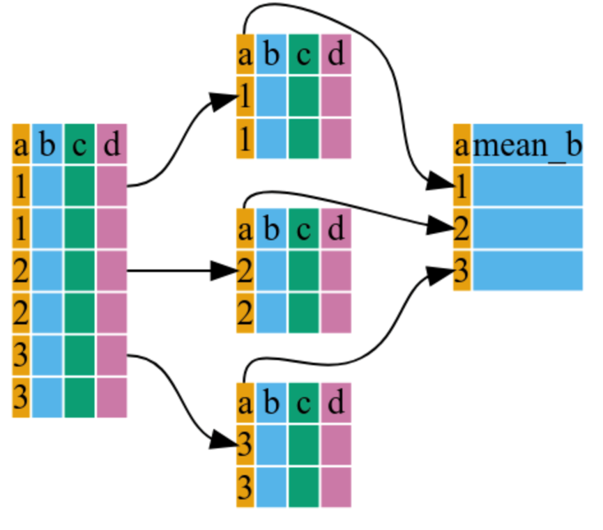
## # ℹ 1,694 more rows

3.2 `summarize()`

This “collapses” each group into a single row of statistics.

# Calculate mean GDP and Standard Error for each continent
gapminder %>% 
  dplyr::group_by(continent) %>% 
  dplyr::summarize(
    mean_le = mean(lifeExp),
    min_le = min(lifeExp),
    max_le = max(lifeExp),
    se_le = sd(lifeExp) / sqrt(dplyr::n()) # n() counts the number of observations
  )
## # A tibble: 5 × 5
##   continent mean_le min_le max_le se_le
##   <fct>       <dbl>  <dbl>  <dbl> <dbl>
## 1 Africa       48.9   23.6   76.4 0.366
## 2 Americas     64.7   37.6   80.7 0.540
## 3 Asia         60.1   28.8   82.6 0.596
## 4 Europe       71.9   43.6   81.8 0.286
## 5 Oceania      74.3   69.1   81.2 0.775

4. `mutate()`: Creating New Variables

mutate() allows you to add new columns while keeping the old ones. It is perfect for calculations like unit conversions or normalization.

# Create a new column for GDP in billions
gapminder %>% 
  dplyr::mutate(gdp_billion = gdpPercap * pop / 10^9) %>% 
  head()
## # A tibble: 6 × 7
##   country     continent  year lifeExp      pop gdpPercap gdp_billion
##   <fct>       <fct>     <int>   <dbl>    <int>     <dbl>       <dbl>
## 1 Afghanistan Asia       1952    28.8  8425333      779.        6.57
## 2 Afghanistan Asia       1957    30.3  9240934      821.        7.59
## 3 Afghanistan Asia       1962    32.0 10267083      853.        8.76
## 4 Afghanistan Asia       1967    34.0 11537966      836.        9.65
## 5 Afghanistan Asia       1972    36.1 13079460      740.        9.68
## 6 Afghanistan Asia       1977    38.4 14880372      786.       11.7

5. Putting It All Together

The true beauty of dplyr is chaining everything into one clean pipeline.

# A complete pipeline: Create a variable, group it, and summarize it
summary_table <- gapminder %>% 
  dplyr::mutate(gdp_billion = gdpPercap * pop / 10^9) %>% 
  dplyr::group_by(continent, year) %>% 
  dplyr::summarize(
    mean_gdpPercap = mean(gdpPercap),
    sd_gdpPercap = sd(gdpPercap),
    mean_pop = mean(pop),
    sd_pop = sd(pop),
    mean_gdp_billion = mean(gdp_billion),
    sd_gdp_billion = sd(gdp_billion)
  )

head(summary_table)
## # A tibble: 6 × 8
## # Groups:   continent [1]
##   continent  year mean_gdpPercap sd_gdpPercap mean_pop   sd_pop mean_gdp_billion
##   <fct>     <int>          <dbl>        <dbl>    <dbl>    <dbl>            <dbl>
## 1 Africa     1952          1253.         983. 4570010.   6.32e6             5.99
## 2 Africa     1957          1385.        1135. 5093033.   7.08e6             7.36
## 3 Africa     1962          1598.        1462. 5702247.   7.96e6             8.78
## 4 Africa     1967          2050.        2848. 6447875.   8.99e6            11.4 
## 5 Africa     1972          2340.        3287. 7305376.   1.01e7            15.1 
## 6 Africa     1977          2586.        4142. 8328097.   1.16e7            18.7 
## # ℹ 1 more variable: sd_gdp_billion <dbl>

Why use dplyr::?

You’ll notice I used dplyr::select() instead of just select(). As we discussed in the “Functions” module, many packages have a filter or select function. Being explicit ensures that your code never breaks, even if you load other libraries later.

0. The “Base R” Struggle (A Scenario)

1. The tidyverse Philosophy

The Power of the Pipe (%>%)

Why use the pipe?

Comparisons: The Pipe vs. The Nest

2. The Core dplyr Verbs

2.1 select(): Picking Columns

2.2 filter(): Picking Rows

3. The Power Duo: group_by() and summarize()

3.1 group_by()

3.2 summarize()

4. mutate(): Creating New Variables

5. Putting It All Together

1. The `tidyverse` Philosophy

The Power of the Pipe (`%>%`)

2. The Core `dplyr` Verbs

2.1 `select()`: Picking Columns

2.2 `filter()`: Picking Rows

3. The Power Duo: `group_by()` and `summarize()`

3.1 `group_by()`

3.2 `summarize()`

4. `mutate()`: Creating New Variables